How to Show Continuous Spectrum Analysis of a Sounf File

In the field of speech analytics, we are required to deal with many of the features available in the audio files. In one of the previous articles, we discussed how to visualize spectrograms and there we went through various insights into any spectrogram related to the audio data. There we also discussed various terminologies and transformations which are required to understand the useful information present in a spectrogram. Proceeding forward, in this article we will get an overview of the various spectral features available in the audio data and how these spectral features can be useful for different aspects of speech and audio analysis. The major points to be discussed in this article are listed in the following table of content.

 Table of Contents

1. Reading the Audio File Using Librosa
2. Chromagram
3. Melspectrogram
4. Mel-Frequency Cepstral Coefficients (MFCCs)
5. Spectral Centroid
6. Spectral RollOff
7. Spectral Bandwidth
8. Spectral Contrast
9. Tonal Centroid Features (Tonnetz)
10. Zero-Crossing Rate

Let's proceed with our discussion.

THE BELAMY

Sign up for your weekly dose of what's up in emerging technology.

Reading the Audio File Using Librosa

In this article, we are going to use the Librosa library for analyzing the audio file and different spectral features.

Importing the libraries

ALSO READ

          import librosa import numpy as np import matplotlib.pyplot as plt from librosa import display from IPython.display import Audio        

In this article, I am using a sample file provided by the Librosa library

Reading audio file,

y, sr = librosa.load(librosa.example('nutcracker'))

Where y is a waveform and we are storing the sampling rate as sr.

In any case with another offline or online file user can use the following code for reading the audio file

y, sr = librosa.load("audio_path")

This code will decompose the audio file as a time series y and the variable sr holds the sampling rate of the time series.

We can listen to the loaded file using the following code.

Audio(data=y,rate=sr)

Output:

Now we can proceed with the further process of spectral feature extraction. To reduce the size of the article, I will be posting only the outputs of the different implementations. For complete codes, you can check out the Google Colab notebook using this link.

Chromagram

Since the word chromatography refers to the separation of different components from its mixture, from here we can understand the meaning of chromagram in the context of audio files. In audio file analysis, an audio file can consist of 12 different pitch classes. These pitch class profiles are very useful tools for analyzing audio files. The term chromagram represents the pitches under an audio file, in one place so that we can understand the classification of the pitches in the audio files. Pitches are the property of any sound or signal which allows the ordering of files based on frequency-related scale. It is some kind of measurement of the quality of the sound which helps in judging the sound as higher, lower, and medium.

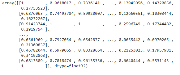
Above we can see the extracted waveform chroma features of the audio file which we have uploaded. These spectral features look better when they get visualized. So next in the article I will visualize them all for better understanding.

There are three types of chromagrams:

• Waveform chromagram – it is basically a chromagram that is computed from the power spectrogram of the audio files. It classifies the waveform of the sound in different pitch classes.
• Constant-Q chromagram– it is a chromagram of constant-Q transform signal. This transformation of the signal takes part in the frequency domain and is related to the Fourier Transform and Morlet Wavelet Transform.
• Chroma energy normalized statistics(CENS) chromagram– as the name suggests this chromagram is made up of signals energy form where furthermore transformation of pitch class by considering short time statistics over energy distribution within the chroma bands helps in obtaining CENS(Chroma energy normalized statistics).

The three types of chromagrams of the audio file which we have imported are represented below.

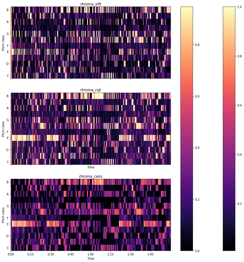
Here we can see here different types of chromagram in which we have used different scales to classify the pitch classes under the audio file. The colours in the graph are showing the different pitch classes between 1 to 12.

Melspectrogram

Mel scale is the scale of pitches that can be felt by the listener to be equal in distance from one another. For example, a listener can identify the difference between the audio of 10000 Hz and 15000 Hz if the audio sources are in the same distance and atmosphere.  Representation of frequencies into the Mel scale generates the Mel spectrogram. Frequencies can be converted into the Mel scale using the Fourier transform.

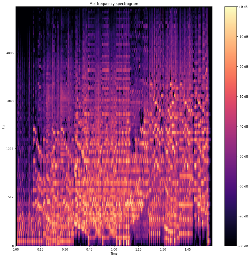
Here in the image, we can see the Mel spectrogram of the sound which we have uploaded wherein the left side frequencies are in the hertz in the right side different Mel scale classes with colours. And how they change according to the pitches.

Mel-Frequency Cepstral Coefficients (MFCCs)

Short term power spectrum of any sound represented by the Mel frequency cepstral (MFC) and combination of MFCC makes the MFC. It can be derived from a type of inverse Fourier transform(cepstral) representation. MFC allows a better representation of sound because in MFC the frequency bands are equally distributed on the Mel scale which approximates the human auditory system's response more closely.

It can be derived by mapping the Fourier transformed signal onto the male scale using triangle or cosine overlapping windows. Where after taking the logs of the powers at each of the Mel frequencies and after discrete cosine transform of the Mel log powers give the amplitude of a spectrum. The amplitude list is MFCC.

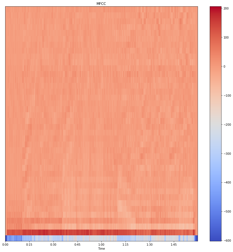
In the above image, we can see the MFCCs of the file which we have uploaded.

Spectral Centroid

As the name suggests, a spectral centroid is the location of the centre of mass of the spectrum. Since the audio files are digital signals and the spectral centroid is a measure that can be useful in the characterization of the spectrum of the audio file signal.

In some places, it can be considered as the median of the spectrum but there is a difference between the measurement of the spectral centroid and median of the spectrum. The spectral centroid is like a weighted median and the median of the spectrum is similar to the mean. Both of them measure the central tendency of the signal. In some cases, both of them show similar results.

Mathematically it can be determined by the Fourier transform of the signals with the weights.

Where

• x(n) is the weight frequency value
• n is the bin number.
• f(n) is the centre frequency of the bin.

Note- we consider the magnitude of the signal as the weight.

Using the spectral centroid we can predict the brightness in an audio file. It is widely used in the measurement of the tone quality of any audio file.

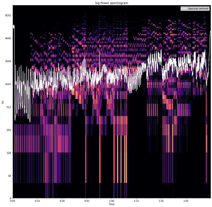
In the above image, the white part shows the centroids of every spectrum and their amplitudes.

Spectral Roll-Off

It can be defined as the action of a specific type of filter which is designed to roll off the frequencies outside to a specific range. The reason we call it roll-off is because it is a gradual procedure. There can be two kinds of filters: hi-pass and low pass and both can roll off the frequency from a signal going outside of their range.

more formally we can say The spectral roll-off point is the fraction of bins in the power spectrum at which 85% of the power is at lower frequencies

This can be used for calculating the maximum and minimum by setting up the roll percent to a value close to 1 and 0.

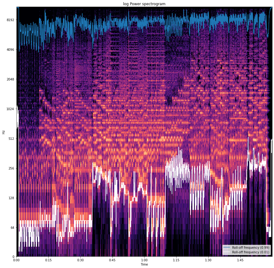
Here in the above image, we can see the hi-pass roll-off as in blue line and low pass roll-off in white colour.

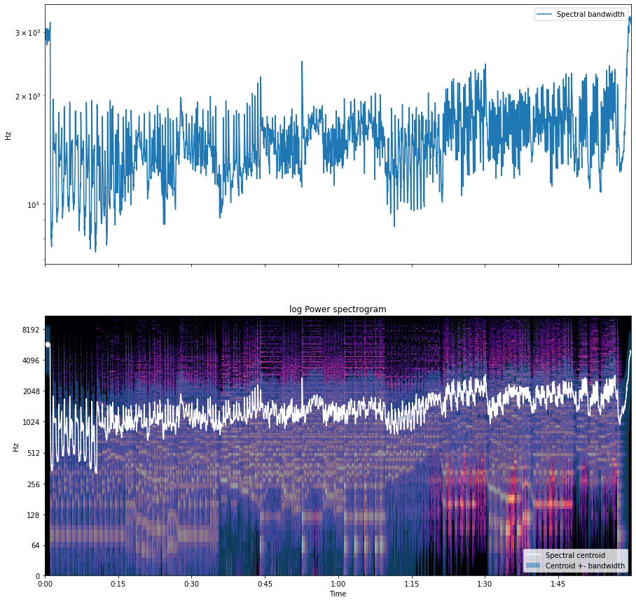
Spectral Bandwidth

Bandwidth is the difference between the upper and lower frequencies in a continuous band of frequencies. As we know the signals oscillate about a point so if the point is the centroid of the signal then the sum of maximum deviation of the signal on both sides of the point can be considered as the bandwidth of the signal at that time frame.

The spectral bandwidth can be computed by

(sum_k S[k, t] * (freq[k, t] - centroid[t])**p)**(1/p)

Where p is order and t is time.

For example, if a signal has frequencies of 1000 Hz, 700 HZ, 300hz, and 100hz then the bandwidth of the signal will be

1000-100 = 900hz.

In the below image we are seeing the magnitude of the bandwidth and in the spectrogram, the blue area is showing the largest deviation of the signal at every time frame by covering the area from blue colour.

Spectral Contrast

In an audio signal, the spectral contrast is the measure of the energy of frequency at each timestamp. Since most of the audio files contain the frequency whose energy is changing with time. It becomes difficult to measure the level of energy. Spectral contrast is a way to measure that energy variation.

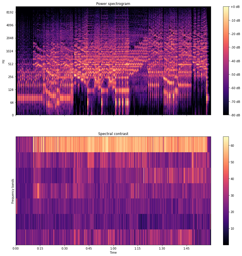
The above image represents the spectral contrast of the file which we have uploaded and also the power spectrum of the audio in different time frames. High contrast values generally correspond to clear, narrow-band signals, while low contrast values correspond to broad-band noise. Here the energy contrast is measured by comparing the mean energy in the peak energy frame to that of the bottom or valley energy frame.

 Tonal Centroid Features (Tonnetz)

As we have seen in the chroma feature part of the article an audio file can consist, 12 pitch classes, this phenomenon considers that the audio file is of 6 pitch classes by merging some of the classes together so the drawn chroma feature graph from this method classifies the pitches only in 6 classes which we call Tonnetz.

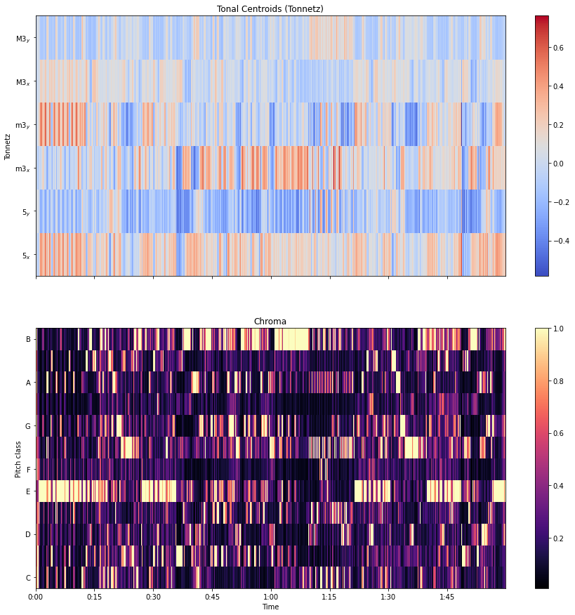
 In the above image, we can see that in our audio file according to the chromagram we have 7 pitch classes but in the tonal centroids we have only 6 pitch classes and accordingly, it has classified the pitches.

Zero-Crossing Rate

As the name suggests zero-crossing rate is the measure of the rate at which the signal is going through the zeroth line more formally signal is changing positive to negative or vice versa.

Mathematically it can be measured as

Where

• s = signal
• T = length of signal

It can be used for pitch detection algorithms and also for voice activity detection.

The file which we have uploaded has a zero-crossing rate of 555.

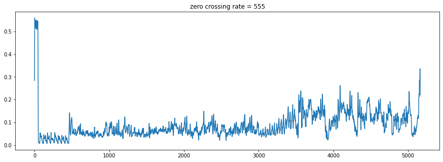
In the above image, we can see the zero cross of our file.

Final Words

Here in the article, we have seen different spectral features which can be extracted according to the requirement for speech and audio data analysis. In the Colab notebook, I have implemented all the codes which anyone can use for their requirements. I encourage readers to go deeper into the subject and implement things in real-life projects.

References:

• Spectral features in Librosa.
• Google Colab notebook for codes.

sampsonfrobeek.blogspot.com

Source: https://analyticsindiamag.com/a-tutorial-on-spectral-feature-extraction-for-audio-analytics/

Share this post